black-hole
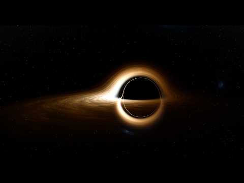
Black Hole Simulation

A real-time, GPU-accelerated browser visualization of a black hole with an accretion flow, jet models, and relativistic optical effects. Runs entirely in the browser using WebGL and three.js.
Live Demo — Chrome or Firefox on a dedicated GPU recommended.
This is a substantially extended fork of oseiskar/black-hole. See What’s new for a summary of additions.
Scientific scope: Schwarzschild photon geodesics follow the exact Binet equation, but rendered fidelity still depends on the integrator, step budget, and adaptive stepping. Spin, accretion, jet, and GRMHD-related options use a mix of analytic, semi-analytic, and heuristic approximations; returning radiation is not ray-traced, and jet colours use an effective-temperature proxy rather than a frequency-resolved synchrotron spectrum. See docs/physics.html for what is exact and what is approximate.
Features
Physics & Rendering
- Two public spin modes —
Fast (Binet lensing)traces photons with the Schwarzschild Binet solver (exact for a = 0) plus perturbative spin heuristics;Kerr-inspired disk velocitieskeeps the same approximate photon solver but uses Kerr equatorial angular velocity to drive disk matter - Three accretion disk models — thin disk (Shakura–Sunyaev), thick torus (ADAF/RIAF), and slim disk (super-Eddington)
- GRMHD-inspired accretion controls — plasma beta (β), magnetic-field strength,
R_highelectron-heating / Ti:Te proxy controls, MAD/SANE magnetic flux, MRI-inspired turbulence, and kappa-distribution electron parameters - Relativistic effects — gravitational redshift, Doppler shift, thermal/background beaming controls (physical D³ Liouville or cinematic), aberration, time dilation
- Relativistic jets — simple analytic jet or a more detailed GRMHD-inspired jet model with spine/sheath structure, reconfinement shocks, jet-corona connection, and Blandford–Znajek-inspired power scaling
- Black-body spectrum — temperature-dependent disk coloring with precomputed Planck lookup
- Multiple tone-mapping modes — ACES Filmic, AgX, and Scientific (logarithmic inferno colormap)
- Multi-pass bloom — threshold → mip-chain Gaussian blur → weighted composite
Post-Processing & Quality
- Temporal Anti-Aliasing (TAA) — history accumulation with motion rejection and clip-box clamping for cleaner still frames
- Six quality presets — Mobile, Optimal, Medium, High, Ultra, and Cinematic
- Auto GPU benchmark — measures frame time on first load and keeps Optimal on capable systems or falls back to Mobile
User Interface
- dat.GUI control panel — resizable right-side panel with collapsible folders for every parameter
- Astrophysical presets — literature-inspired starting points for M87*, Sgr A*, Cygnus X-1, GRS 1915+105, and more
- Observer controls — mouse orbit/pan/roll, a bottom-left observer widget with distance dial + motion toggle, and optional automatic circular orbit in the stable Schwarzschild regime (
r >= 3 r_s)
Presentation & Recording
- Presentation Timeline — bottom-docked dopesheet editor (inspired by Blender / After Effects) for scripted keyframe animations, preset loading, playback, and recording; supports linear, smooth, and smoother easing
- Built-in interactive scenarios — Freefall Dive and Hover Approach
- Live scenario capture to timeline — record a manual Freefall Dive or Hover Approach run, including orbit/pan camera motion and captured shader time, straight into timeline tracks, with optional camera smoothing
- Built-in timeline presets — Full Feature Tour (186 s) and Orbit Showcase
- WebM video recording — realtime MediaRecorder capture plus offline WebCodecs/WebM muxing when supported
- Offline PNG snapshot — one-click still export that forces the Cinematic (offline) quality preset before download
- High-quality offline rendering — Cinematic preset with manually boosted supersampling for publication-quality stills and video frames
Physics Documentation
See docs/physics.html for a detailed description of the models, equations, approximations, and implementation scope used in the simulation, with academic references and notes on where the renderer departs from full GRRT/GRMHD treatments.
Quick Start
Clone or download this repository, then launch a local HTTP server:
python -m http.server 8000
Open http://localhost:8000 in a modern browser (Chrome or Firefox recommended). A dedicated GPU is recommended for smooth rendering.
Performance tips
| Action | Effect |
|---|---|
| Lower quality preset (GUI → Quality) | Reduces integration steps and supersampling |
| Shrink the browser window | Fewer pixels to trace |
| Disable the planet | Removes ray-sphere intersection tests |
| Disable RK4 | Falls back to leapfrog / Störmer-Verlet integration (faster, less accurate near the photon sphere) |
| Switch solver mode to Fast | Uses the lightweight Binet photon solver everywhere |
Controls
- Left drag — orbit the camera
- Right drag — pan
- Left + Right drag — roll
- Scroll — zoom in/out
- Controls panel (right side,
CONTROLS ▶) — all simulation parameters - Animations panel (left side,
◀ ANIMATIONS) — Freefall Dive, Hover Approach, and live capture of those runs into the timeline - Observer widget (bottom-left XYZ indicator) — distance dial, motion toggle, camera reset
- Timeline panel (bottom,
▲ TIMELINE) — preset loading, timeline editing, playback, recording, and export/import
Key GUI parameters
| Parameter | Description |
|---|---|
| a/M | Signed black hole spin; positive and negative values mirror the spin direction |
| solver mode | Fast (Binet lensing) or Kerr-inspired disk velocities; the latter keeps approximate photon lensing but uses Kerr angular velocity to drive disk matter |
| temperature (K) | Visualized disk color temperature in Kelvin (4,500 – 30,000 K) |
| disk model | Thin disk, thick torus (ADAF), or slim disk |
| doppler shift (color) | Toggle relativistic red/blue spectral shifting for black-body-based thermal emitters and the background-sky proxy; jets keep their own synchrotron-motivated transfer |
| physical (D³ Liouville) | Use physically motivated beaming for thermal emitters and the background-sky proxy instead of the softened cinematic curve |
| jet enabled / mode | Toggle jets and choose simple or more detailed GRMHD-inspired shading |
| observer motion | Toggle automatic circular orbit around the black hole; motion is clamped to the stable Schwarzschild regime (r >= 3 r_s) |
| quality preset | Mobile / Optimal / Medium / High / Ultra / Cinematic |
Quality preset levels
| Preset | Steps (fast / Kerr-inspired) | Supersampling | Description |
|---|---|---|---|
| Mobile | 28 / 120 | 1× | 0.55× resolution + TAA; fastest |
| Optimal | 100 / 400 | 1× | 0.8× res + TAA; recommended default |
| Medium | 100 / 400 | 1× / 3× | Full resolution; balanced |
| High | 320 / 520 | 4× | Full resolution; GPU-intensive |
| Ultra | 600 / 1400 | 4× / 6× | Maximum fidelity |
| Cinematic | 600 / 1400 | 6x / 12x | Offline rendering quality |
Built-in black hole presets
| Preset | Object | Notes |
|---|---|---|
| Default | Generic BH | a/M = 0.90, thin disk |
| M87* | Virgo A SMBH | Illustrative high-spin, MAD-like thick-torus + jet configuration inspired by EHT-era GRMHD studies |
| Sgr A* | Milky Way centre | Illustrative moderate-spin ADAF/RIAF-style torus; EHT modeling does not determine a unique spin |
| Cygnus X-1 | X-ray binary | Near-extremal thin-disk preset inspired by continuum-fitting studies |
| GRS 1915+105 | Microquasar | Near-extremal slim-disk preset inspired by continuum-fitting and jet observations |
| Gargantua (Interstellar visuals) | Film-inspired | Warm thin disk, boosted glow, softened relativistic effects |
| Schwarzschild | Textbook case | Spin disabled, clean circular shadow |
How It Works
- Each screen pixel casts a ray from the camera into the scene.
- The ray direction is transformed for relativistic aberration if the observer is moving.
- Photon paths are traced with the Schwarzschild Binet equation (leapfrog / RK4). The optional
Kerr-inspired disk velocitiesmode keeps the same photon solver but upgrades disk matter to a Kerr-inspired orbital-velocity model. - At each step, intersections with the accretion disk, GRMHD-inspired media, jets, and planet are tested and composited using Beer–Lambert transmittance.
- Doppler shift, gravitational redshift, and beaming are applied with model-appropriate transfer rules; jets use a separate synchrotron-motivated treatment.
- The background sky (Milky Way panorama + star field) is rendered with optional Doppler color shifting.
- The HDR accumulation buffer is bloom-composited and then tone-mapped to sRGB.
- Optionally, TAA accumulates multiple jittered frames before display.
Project Structure
The codebase is organized into logical modules by function and responsibility.
GLSL Shaders (shaders/raytracer/)
shaders/raytracer/
├── core/                          # Foundational definitions
│   ├── defines.glsl              # Constants, macros, uniforms, rendering params
│   └── math.glsl                 # Math utilities, coordinate transforms, FBM noise
├── physics/                       # Physics models
│   ├── geodesics.glsl            # Schwarzschild Binet solver + experimental Kerr Mino-time helpers
│   ├── accretion.glsl            # Thin disk, ADAF torus, slim disk, GRMHD-inspired turbulence
│   ├── jet.glsl                  # Jet models: simple parabolic + more detailed GRMHD-inspired mode
│   ├── planet.glsl               # Planet ray-sphere intersection
│   └── background.glsl           # Galaxy/star background rendering
└── output/                        # Rendering pipeline
    ├── tonemapping.glsl          # ACES Filmic, AgX, scientific tone-mappers
    ├── trace_ray.glsl            # Core ray-marching loop with Beer-Lambert composite
    └── main.glsl                 # GLSL main() entry point
JavaScript Modules (js/app/)
js/app/
├── bootstrap.js                    # Entry point: fetches GLSL shards & textures, calls init()
├── core/                           # System core
│   ├── observer.js                 # Observer state, circular-orbit kinematics, simulation time scaling
│   ├── shader.js                   # Shader class, compile-time Mustache parameters
│   └── renderer.js                 # Three.js scene, live dive/hover capture, TAA, bloom, render loop
├── scene/                          # Scene management
│   └── camera.js                   # Camera initialization & per-frame updates
├── graphics/                       # Graphics effects
│   └── bloom.js                    # Multi-pass mip-chain Gaussian bloom
├── presentation/                   # Presentation & recording system
│   ├── presentation-controller.js  # Keyframe timeline engine, annotations, recording pipeline
│   ├── presentation-gui.js         # Legacy presentation mini-panel helper (kept for reference)
│   ├── timeline-panel.js           # Bottom dopesheet panel (transport, presets, key inspector, recording)
│   └── presets/                    # Built-in animation sequences (JSON)
│       ├── manifest.json
│       ├── full-feature-tour.json
│       └── orbit-showcase.json
└── ui/                             # User interface
    ├── presets.js                  # Astrophysical black hole preset library
    ├── quality-presets.js          # Rendering quality preset library
    └── gui.js                      # dat.GUI panel setup and parameter wiring
Other files
index.html                          # Web page entry point
style.css                           # Styling (panels, timeline, controls)
three-js-monkey-patch.js            # Legacy Three.js compatibility patches
js-libs/                            # Third-party libraries (three.js, dat.GUI, webm-muxer, …)
docs/
├── physics.html                    # Comprehensive physics documentation
├── presentation-editor.md          # Guide to using the presentation timeline editor
└── presentation-json.md            # Timeline JSON schema & advanced event guide
What’s New in This Fork
Additions over the upstream oseiskar/black-hole:
| Feature | Details |
|---|---|
| WIP Kerr geodesics | Carter (1968) Mino-time integrator exists in GLSL but is not yet exposed in the UI |
| GRMHD-inspired accretion controls | plasma β, B-field strength, R_high, MAD flux, MRI-inspired turbulence, κ-distribution electrons |
| Presentation Timeline | Keyframe dopesheet editor with presets, transport controls, recording, and easing curves |
| Scenario capture to timeline | Records live Freefall Dive / Hover Approach runs plus camera motion into keyframed timeline data |
| WebM recording | Realtime MediaRecorder capture plus offline WebCodecs/WebMMuxer export |
| Offline PNG snapshot | One-click still image export using the Cinematic offline preset |
| Interactive observer scenarios | Freefall Dive and Hover Approach |
| Built-in timeline presets | Full Feature Tour and Orbit Showcase |
| Astrophysical BH presets | M87*, Sgr A*, Cygnus X-1, GRS 1915+105, Gargantua, Schwarzschild |
| Temporal Anti-Aliasing | Motion-rejection TAA for cleaner high-quality frames |
| Six quality tiers | Mobile, Optimal, Medium, High, Ultra, Cinematic |
| Three tone-mappers | ACES Filmic, AgX, Scientific (inferno colormap) |
| Three accretion models | Thin disk, thick torus (ADAF), slim disk (super-Eddington) |
| GRMHD-inspired jet model | Spine/sheath, reconfinement shocks, Blandford–Znajek-inspired power scaling |
| Resizable UI panels | Drag-to-resize controls panel and timeline |
License
The source code for this fork is MIT-licensed, but the repository as distributed is a mixed-license bundle. Some bundled third-party libraries and assets use separate terms, and the shipped Milky Way panorama is not covered by the MIT code license. See COPYRIGHT.md for the full breakdown. If you need a clean permissive redistribution, replace the restricted third-party assets first.
Originally based on oseiskar/black-hole (MIT).
Fork maintained and substantially extended by Adriwin.
AI Disclaimer: AI assisted with translating complex general-relativity equations into functional WebGL shaders and with structuring academic references. The original codebase was human-made and well-written. The main physics formulas, approximations, and external references are documented in docs/physics.html.
Demo